Data Assimilation¶

In this section, we discuss the current implementation of the Data Assimilation and the usage of the assim command line interface.

Introduction¶

The idea is to combine the best different sources of information to estimate the state of a system:

model equations

observations, data

background, a priori information

statistics

In our specific application, we combine our hydrological model with stream flow observations.

In the following sections, the Top Layer Hydrological Model will be used to illustrate the theory of data assimilation.

Best Linear Unbiased Estimator (BLUE)¶

We aim at producing an estimate \(x^a\) of the true state \(x^t=(q,S_p,S_t,S_s)\) of the hillslope/river network at initial time, to initialize forecasts.

We are given:

a background estimate \(x^b=(q^b,S_p^b,S_t^b,S_s^b)\) with covariance matrix \(B\) given, from a previous forecast,

partial observations \(y^0=\mathcal{H}(x^t)+\varepsilon^0\), with covariance matrix \(R\) given, e.g. water elevation from bridge sensors. Observation operator \(\mathcal{H}\) maps the input parameters to the observation variables, in our case it would be the rating curves.

We also assume that:

\(\mathcal{H} = H\) is a linear operator

The best estimate \(x^a\) is searched for as a linear combination of the background estimate and the observation \(y^o\):

\[x^a = L x^b + K y^o\]

Variational method¶

We can rewrite the BLUE as an equivalent variational optimization problem (optimal least squares) also :

\[x^a = min(\mathcal{J})\]

where the cost function \(\mathcal{J}\) to minimize is:

\[\mathcal{J}(x) = (x-x^b)^T B^{-1} (x-x^b) + (y^o -H(x))^T R^{-1}(y^o-H(x))\]

Let’s introduce a model operator:

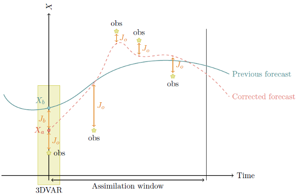
\[x_k^t = \mathcal{M}_{k,k-1}(x_{k-1}^t) = \mathcal{M}_{0 \to k}(x_0^t)\]

Since our problem is time-dependant (4D-Var), and the unknown x is the initial state vector:

\[\mathcal{J}(x) = \underbrace{(x-x^b)^T B^{-1} (x-x^b)}_{\mathcal{J}_b} + \underbrace{(y^o -H_k(\mathcal{M}_{0 \to k}(x)))^T R^{-1}(y^o -H_k(\mathcal{M}_{0 \to k}(x)))}_{\mathcal{J}_o}\]

Where \(\mathcal{J}_b\) to minimize the distance to the a priori information and \(\mathcal{J}_o\) minimize the distance to the observations.

This is illustrated in the following figure:

Now that \(\mathcal{J}\) is defined (i.e. once all the ingredients are chosen: control variables, error statistics, norms, observations…), the problem is entirely defined. Hence its solution. To minimize \(\mathcal{J}\) we will be using a descent method:

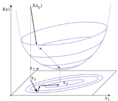
Descent methods to minimize a function require knowledge of (an estimate of) its gradient. Obtaining the gradient through the computation of growth rates is unpractical since it require N + 1 runs, where \(N = [x]\). In our state wide application, \(N = O(7)\).

There are two typical methods to get an estimate of the gradient with one run of the model:

Adjoint model

Forward Sensitivity equations

The later is used in this implementation and sensitivity to background equations are solved along the model equations.

Forward Sensitivity Methods (FSM)¶

TODO: show relation between \(\nabla{\mathcal{J}(x)}\) and FSM.

Problem simplification¶

Although the equations are numerous, and the corresponding least squares problem requires solving linear systems of equations, several observations can be made to reduce the overall workload:

Ungagged sub-basin are removed

Zone of influence is defined as an area upstream the gage that has an influence on the discharge at gage during the assimilation window. For that we use constant streamflow velocity to assess the maximum distance

Installation¶

Data Assimilation is available only if Asynch is built with the PETSc library. Refer to the Installation for more information. Make sure that ./configure returns:

checking for PETSC... yes

Configuration¶

assim requires an additional configuration .das file on the command line, for exemple:

assim turkey_river.gbl turkey_river.das

Overview¶

Here is a typical .das file taken from the examples folder:

%Model variant
254_q

%Observation input (discharge)
%Time resolution of observations
assim51.dbc 15.0

%Step to use (assimilation window)
%12 % use 3 hours
%24 % use 6 hours
48 % use 12 hours
%96 % use 24 hours

%Max least squares iterations
5

# %End of file
-------------------------------

Model variant¶

Format:

{model id}

This string value specifies which assimilation model is used and which state variable initial conditions are optimized.

Id	Model	State variable
254	Top Layer Model	Every state variable
254_q	Top Layer Model	Discharge
254_qsp	Top Layer Model	Discharge, pond storage
254_qst	Top Layer Model	Discharge, top layer storage

Observation input¶

Format:

{.dbc filename} {time resolution}

The observation data are pulled from a PostgreSQL database. The database connection filename can include a path. The file should provide three queries in the following order:

A query that returns the link_id where observation (gages) are available with the following schema CREATE TABLE (link_id integer).

A query that returns observation for a given time frame (where begin and end time stamp are parameter) with the following schema CREATE TABLE (link_id integer, datetime as integer, discharge real).

A query that returns the distance to the border of the domain for the gages with the following schema CREATE TABLE (link_id integer, distance real).

The time resolution is a floating point number with units in minutes.

Assimilation Window¶

Format:

{num observations}

The duration of the assimilation window expressed in number of time steps.

Forecaster¶

Running a forescaster with data assimilation requires to run a background simulation with asynch followed by the analysis with assim. And then generate the forecast using the analysed state as initial conditions. Here are the typical steps to

First the model needs to be intialized, for instance, with hydrostatic conditions. Given the discharge at the outlet \(q\) and the draining area \(\mathcal{A}\), compute the equivalent precipitation \(p_{eq}\) and using dry uniform intial condition run the model for a long period with the equivalent precipitation. This will fill up the watershed.

\[p_{eq} = \frac{q}{\mathcal{A}}\]

Then run a warmup period of 15 days (or wathever the travel time is for your waterhed) with real precipitation data. At this point we should have realistic initial conditions.
Finally run the following algorithm:

ON discharge_observation
  // Generate the background
  RUN asynch for obs time step

  // Generate the assimilated state
  RUN assim for the assimiliation window

  // Generate forecast
  RUN asynch for the forecast lead time

Here is a snippet of an implementation of this algorithm in Javascript:

//Get the initial condition file (the timestamp is in the filename)
var file = getLatestFile(/^background_(\d+).(rec|h5)$/);

//Main time loop
while (file.timestamp < endTime) {

  // Assimilation window
  const assim_window = 12 * 60

  // Steps of 6 hours
  const duration = 6 * 60;

  // Generate the config file for DA
  render(templates.assim, 'assim.gbl', {
    duration: assim_window,
    begin: file.timestamp,
    end: file.timestamp + assim_window * 60
  });

  cp.execFileSync('mpiexec', ['-n', '4', 'assim', 'assim.gbl', 'assim.das'], {stdio:[0,1,2]});

  // Generate the config file for the background (regular asynch run)
  render(templates.background, 'background.gbl', {
    duration: duration,
    begin: file.timestamp,
    end: file.timestamp + duration * 60
  });

  cp.execFileSync('mpiexec', ['-n', '1', 'asynch', 'background.gbl'], {stdio:[0,1,2]});

  file.timestamp += duration * 60;
}

The full implementation is available in the examples/assim folder.

Notes¶

Note

The author of these docs is not the primary author of the code so some things may have been lost in translation.

Data assimilation is implemented only for the Top Layer Hydrological Model (254). Implementing Data Assimilation requires the user to provide additional model’s equations. A more generic method could be used (Jacobian approximation) but would probably be less efficient.

Data assimilation only works with discharge observations (or whatever the first state variable is). This is currently hardcoded but could be extended to support other types of observation such as soil moisture.

Observations should be interpolated to get a better assimilated states (especially for locations that are close to observations). For instance with discharge observations available at a 15 minutes time step, links that are upstream at a distance \(d < 15 * v_0\) are not corrected.

The larger the assimilation window, the larger is the domain of influence upstream the gages and the better the corrected state. A short assimilation window would only make correction to the links close to the gage and that could induce some ossilations. In Iowa 12 hours, seems to be the sweet spot between computation time and correction.

The solution of the equations at a link depends on the upstreams links and not only the direct parent links. This difference between the forward model and the assimilation model makes Asynch less suitable for solving the system of equations. To be more specific, the partionning of the domain between processors is more senstive since a bad partionning may results in a lot a transfers between procs. Eventually a solver like CVODES (Sundials), that solves the sensitivity equations, may be more appropriate.

For small watersheds (N <= 15K links, i.e. Turkey River), assim works best using serial execution (num procs = 1).

The performances of the assimilation are not very good when the correction of discharge is negative (falling limb).

Discontinuities (i.e. at reservoirs) are not supported.

Strong nonlinearities could be problem. The extension of 4D-Var to non linear problems, called Incremental 4D-Var, may be more appropriate.

Bibliography¶

[da]	Maelle Nodet, “Introduction to Data Assimilation”, Université Grenoble Alpes, Mars 2012

[fs]	Lakshmivarahan and J. M. Lewis, “Forward Sensitivity Approach to Dynamic Data Assimilation”, Advances in Meteorology, vol. 2010, Article ID 375615, 12 pages, 2010. doi:10.1155/2010/375615

[grad]

Sengupta, B., K.J. Friston, and W.D. Penny. “Efficient Gradient Computation for Dynamical Models.” Neuroimage 98.100 (2014): 521–527. PMC. Web. 10 July 2017.