Built-in Models
| Model Type | Description | States |
|---|---|---|
| 21 | Linear reservoir model, with dams | \(q\), \(S\), \(S_s\), \(S_g\) |
| 40 | Linear reservoir model, with qvs dams | \(q\), \(S\), \(S_s\), \(S_g\) |
| 190 | IFC linear model with constant runoff | \(q\), \(s_p\), \(s_s\) |
| 191 | IFC linear model with constant runoff | \(q\), \(s_p\), \(s_s\), \(s_{precip}\), \(V_r\), \(q_b\) |
| 192 | IFC linear model with variable runoff | \(q\), \(s_p\), \(s_s\), \(s_{precip}\), \(V_r\), \(q_b\) |
| 195 | IFC linear model, offline precip. | \(q\), \(s_p\), \(s_s\), \(s_{precip}\) |
| 196 | IFC linear model, offline precip. | \(q\), \(s_p\), \(s_s\), \(s_{precip}\), \(s_{runoff}\) |
| 252 | IFC toplayer model | \(q\), \(s_p\), \(s_t\), \(s_s\) |
| 253 | IFC toplayer model, with reservoirs | \(q\), \(s_p\), \(s_t\), \(s_s\) |
| 254 | IFC toplayer model, with reservoirs | \(q\), \(s_p\), \(s_t\), \(s_s\), \(s_{precip}\), \(V_r\), \(q_b\) |
| 256 | IFC toplayer model with interflow | \(q\), \(s_p\), \(s_t\), \(s_s\), \(s_{precip}\), \(s_{evap}\), \(s_{runoff}\), \(q_b\) |
| 257 | IFC toplayer model, variable velocity | \(q\), \(s_p\), \(s_t\), \(s_s\), \(s_{precip}\), \(s_{et}\), \(V_r\), \(q_b\) |
| 258 | IFC toplayer model, offline precip. | \(q\), \(s_p\), \(s_t\), \(s_s\), \(s_{precip}\), \(s_{evap}\), \(s_{runoff}\), \(q_b\) |
| 259 | IFC toplayer with offline, interflow | \(q\), \(s_p\), \(s_t\), \(s_s\), \(s_{precip}\), \(s_{evap}\), \(s_{runoff}\), \(q_b\) |
In this section, a description of a few different models is presented to demonstrate the features described in Section [sec: model descriptions]. These models are already fully implemented in problems.c and definetype.c, and may be used for simulations.
Main models
Constant Runoff Hydrological Model
This model describes a hydrological model with linear reservoirs used to describe the hillslope surrounding the channel. This is equivalent to a hillslope with a constant runoff. This model is implemented as model 190.
Three states are modeled at every link:
| State | Description |
|---|---|
| \(q(t)\) | Channel discharge [\(m^3/s\)] |
| \(s_p(t)\) | Water ponded on hillslope surface [\(m\)] |
| \(s_s(t)\) | Effective water depth in hillslope subsurface [\(m\)] |
where each state is a function of time (\(t\)), measured in \(mins\).
These states are given as the solution to the differential equations
Here, precipitation and potential evaporation are given as the time series \(p(t)\) and \(e_{pot}(t)\), measured in \(mm/hr\) and \(mm/month\), respectively. The function \(q_{in}(t)\) is the total discharge entering the channel from the channels of parent links, measured in \(m^3/s\). A flux moves water from the water ponded on the surface to the channel, and another flux moves water from the subsurface to the channel. These are defined by:
Further fluxes representing evaporation are given by:
When potential evaporation is \(0\), the fluxes \(e_p\) and \(e_s\) are taken to be \(0\ m/min\).
Some values in the equations above are constant in time, and are given by:
Several parameters are required for the model. These are constant in time and represent:
| Parameters | Description |
|---|---|
| \(A\) | Total area draining into this link [\(km^2\)] |
| \(L\) | Channel length of this link [\(km\)] |
| \(A_h\) | Area of the hillslope of this link [\(km^2\)] |
Finally, some parameters above are constant in time and take the same value at every link. These are:
| Parameters | Description |
|---|---|
| \(v_r\) | Channel reference velocity [\(m/s\)] |
| \(\lambda_1\) | Exponent of channel velocity discharge [] |
| \(\lambda_2\) | Exponent of channel velocity area [] |
| \(RC\) | Runoff coefficient [] |
| \(v_h\) | Velocity of water on the hillslope [\(m/s\)] |
| \(v_g\) | Velocity of water in the subsurface [\(m/s\)] |
Let’s walk through the required setup for this model. The above information for the model appears in three different source files: definetype.c, problems.c, and problem.h which is pretty bad and will be fix in the near future.
The function SetParamSizes contains the block of code for model 190:
globals->dim = 3;
globals->template_flag = 0;
globals->assim_flag = 0;
globals->diff_start = 0;
globals->no_ini_start = globals->dim;
num_global_params = 6;
globals->uses_dam = 0;
globals->params_size = 8;
globals->iparams_size = 0;
globals->dam_params_size = 0;
globals->area_idx = 0;
globals->areah_idx = 2;
globals->disk_params = 3;
globals->num_dense = 1;
globals->convertarea_flag = 0;
globals->num_forcings = 2;
Each value above is stored into a structure called GlobalVars. Details about this object can be found in GlobalVars. Effectively, this object holds the values described in Section SetParamSizes. dim is set to 3, as this is the number of states of the model (\(q\), \(s_p\), and \(s_s\)). This value is the size of the state and equation-value vectors. For the ordering in these vectors, we use:
This ordering is not explicitly stated anywhere in code. Anytime a routine in definetype.c or problems.c accesses values in a state or equation-value vector, the routine’s creator must keep the proper ordering in mind. template_flag is set to 0, as no XML parser is used for the model equations. assim_flag is set to 0 for no data assimilation.
The constant runoff model consists entirely of differential equations (i.e. no algebraic equations), so diff_start can be set to the beginning of the state vector (index 0). no_ini_start is set to the dimension of the state vector. This means initial conditions for all 3 states must be specified by the source from the global file in the initial values section (see Initial States).
Six parameters are required as input which are uniform amongst all links. This value is stored in num_global_params. This model does use dams, so the uses_dam flag is set to 0 and dam_params_size is set to 0.
Each link has parameters which will be stored in memory. Some of these values must be specified as inputs, while others can be computed and stored. For the constant runoff model, these parameters and the order in which we store them is
Each link has 8 parameters and no integer parameters. Thus params_size is set to 8 and iparams_size is set to 0. The parameters \(A\), \(L\), and \(A_h\) are required inputs, while the others are computed in terms of the first three parameters and the global parameters. Therefore disk_params is set to 3. The index area_idx is set to 0, as 0 is the index of the upstream area. Similarly, areah_idx is set to 2 for the hillslope area. convertarea_flag is set to 0, as the hillslope area will be converted to units of \(m^2\), as shown below.
When passing information from one link to another downstream, only the channel discharge \(q\) is needed. So we set num_dense to 1. Finally, two forcings are used in the constant runoff model (precipitation and evaporation), so num_forcings is set to 2.
In the SetParamSizes routine, an array dense_indices is created with a single element (the size is num_dense). For model 190, the entry is set via:
globals->dense_indices[0] = 0; //Discharge
Because the state \(q\) is passed to other links, its index in state vectors is put into the dense_indices array.
In the routine ConvertParams, two parameters are opted to receive a unit conversion:
params.ve[1] *= 1000;  //L: km -> m
params.ve[2] *= 1e6;   //A_h: km^2 -> m^2
The parameter with index 1 (\(L\)) is multiplied by 1000 to convert from \(km\) to \(m\). Similarly, the parameter with index 2 (\(A_h\)) is converted to \(km^2\) to \(m^2\). Although these conversions are optional, the model differential equations contain these conversions explicitly. By converting units now, the conversions do not need to be performed during the evaluation of the differential equations.
In the routine Precalculations, each of the parameters for the constant runoff model are calculated at each link. The code for the calculations is:
else if(type == 190)
{
  double* vals = params.ve;
  double A = params.ve[0];
  double L = params.ve[1];
  double A_h = params.ve[2];
  double v_r = global_params.ve[0];
  double lambda_1 = global_params.ve[1];
  double lambda_2 = global_params.ve[2];
  double RC = global_params.ve[3];
  double v_h = global_params.ve[4];
  double v_g = global_params.ve[5];

  vals[3] = v_h * L / A_h * 60.0;   //k_2
  vals[4] = v_g * L / A_h * 60.0;   //k_3
  vals[5] = 60.0*v_r*pow(A,lambda_2) / ((1.0-lambda_1)*L); //invtau
  vals[6] = RC*(0.001/60.0);    //c_1
  vals[7] = (1.0-RC)*(0.001/60.0);  //c_2
}
Here, the array of parameters is named vals (simply as an abbreviation). The input parameters of the system are extracted (with the conversions from ConvertParams), and the remaining parameters are calculated, and saved into the corresponding index in params.
In the routine InitRoutines, the Runge-Kutta solver is selected based upon whether an explicit or implicit method is requested:
else if(exp_imp == 0)
  link->RKSolver = &ExplicitRKSolver;
else if(exp_imp == 1)
  link->RKSolver = &RadauRKSolver;
Other routines are set here:
else if(type == 190)
{
  link->f = &LinearHillslope_MonthlyEvap;
  link->alg = NULL;
  link->state_check = NULL;
  link->CheckConsistency =
  &CheckConsistency_Nonzero_3States;
}
The routines for the algebraic equations and the system state check are set to NULL, as they are not used for this model. The routines for the differential equations and state consistency are found in problems.c. The routine for the differential equations is LinearHillslope_MonthlyEvap:
void LinearHillslope_MonthlyEvap
(double t,VEC* y_i,VEC** y_p,
unsigned short int numparents,VEC* global_params,
double* forcing_values,QVSData* qvs,VEC* params,
IVEC* iparams,int state,unsigned int** upstream,
unsigned int* numupstream,VEC* ans)
{
  unsigned short int i;

  double lambda_1 = global_params.ve[1];

  double A_h = params.ve[2];
  double k2 = params.ve[3];
  double k3 = params.ve[4];
  double invtau = params.ve[5];
  double c_1 = params.ve[6];
  double c_2 = params.ve[7];

  double q = y_i.ve[0];      //[m^3/s]
  double s_p = y_i.ve[1];    //[m]
  double s_s = y_i.ve[2];    //[m]

  double q_pc = k2 * s_p;
  double q_sc = k3 * s_s;

  //Evaporation
  double C_p,C_s,C_T,Corr_evap;
  double e_pot = forcing_values[1] * (1e-3/(30.0*24.0*60.0)); //[mm/month] -> [m/min]

  if(e_pot > 0.0)
  {
    C_p = s_p / e_pot;
    C_s = s_s / e_pot;
    C_T = C_p + C_s;
  }
  else
  {
    C_p = 0.0;
    C_s = 0.0;
    C_T = 0.0;
  }

  Corr_evap = (C_T > 1.0) ? 1.0/C_T : 1.0;

  double e_p = Corr_evap * C_p * e_pot;
  double e_s = Corr_evap * C_s * e_pot;

  //Discharge
  ans.ve[0] = -q + (q_pc + q_sc) * A_h/60.0;
  for(i=0;i<numparents;i++)
  ans.ve[0] += y_p[i]->ve[0];
  ans.ve[0] = invtau * pow(q,lambda_1) * ans.ve[0];

  //Hillslope
  ans.ve[1] = forcing_values[0]*c_1 - q_pc - e_p;
  ans.ve[2] = forcing_values[0]*c_2 - q_sc - e_a;
}
The names of parameters and states match with those defined in the mathematics above. The current states and hillslope parameters are unpacked from the state vector y_i and the vector params, respectively. The current precipitation value is available in forcing_values[0] and the current potential evaporation is available in forcing_values[1]. The fluxes \(q_{pc}\) and \(q_{sc}\) are calculated and used as q_pc and q_sc, respectively. The evaluation of the right side of the differential equations is stored in the equation-value vector ans. The channel discharges for the parent links are found in the array of state vectors y_p[i]->ve[0], with i ranging over the number of parents.
The state consistency routine for the constant runoff model is called CheckConsistency_Nonzero_3States. It is defined as:
void CheckConsistency_Nonzero_3States(VEC* y,
VEC* params,VEC* global_params)
{
  if(y.ve[0] < 1e-14)    y.ve[0] = 1e-14;
  if(y.ve[1] < 0.0)  y.ve[1] = 0.0;
  if(y.ve[2] < 0.0)  y.ve[2] = 0.0;
}
The hillslope states \(s_p\) and \(s_s\) should not take negative values, as each is a linear reservoir. Similarly, the channel discharge \(q\) decays to 0 exponentially as the fluxes from the hillslope and upstream links goes to 0. However, because of the dependence upon \(q^{\lambda_1}\) in the equation for \(\frac{dq}{dt}\), \(q\) must be kept away from 0. We therefore force it to never become smaller than \(10^{-14}\ m^3/s\). It is worth noting that this restriction on \(q\) can only work if the absolute error tolerance for \(q\) is greater than \(10^{-14}\ m^3/s\).
Each of these functions must also be declared in problems.h:
void LinearHillslope_MonthlyEvap(double t,VEC* y_i,  VEC** y_p,unsigned short int numparents,  VEC* global_params,double* forcing_values,  QVSData* qvs,VEC* params,IVEC* iparams,  int state,unsigned int** upstream,  unsigned int* numupstream,VEC* ans);
void CheckConsistency_Nonzero_3States(VEC* y,  VEC* params,VEC* global_params);
The routine ReadInitData only needs to return a value of 0 for model 190. All states are initialized from through a global file, as no algebraic equations exist for this model, and no_ini_start is set to dim. No state discontinuities are used for this model, so a value of 0 is returned.
Top Layer Hydrological Model
This model describes a hydrological model with nonlinear reservoirs used to describe the hillslope surrounding the channel. It features a layer of topsoil to create a runoff coefficient that varies in time. This model is implemented as model 254. The setup of the top layer model is similar to that of the constant runoff model presented in Section Constant Runoff Hydrological Model. However, the top layer model does make use of additional features.
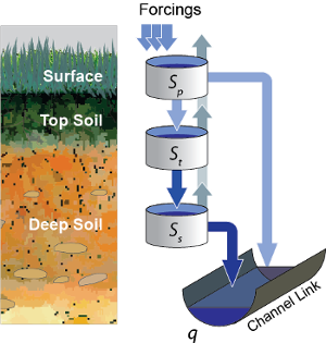
The top layer hillslope model
Seven states are modeled at every link:
| State | Description |
|---|---|
| \(q(t)\) | Channel discharge [\(m^3/s\)] |
| \(s_p(t)\) | Water ponded on hillslope surface [\(m\)] |
| \(s_t(t)\) | Effective water depth in the top soil layer [\(m\)] |
| \(s_s(t)\) | Effective water depth in hillslope subsurface [\(m\)] |
| \(s_{precip}(t)\) | Total fallen precipitation from time \(0\) to \(t\) [\(m\)] |
| \(V_r(t)\) | Total flux of water from runoff from time \(0\) to \(t\) [\(m^3/s\)] |
| \(q_b(t)\) | Channel discharge from baseflow [\(m^3/s\)] |
where each state is a function of time (\(t\)), measured in \(mins\).
These states are given as the solution to the differential equations
Here, precipitation and potential evaporation are given as the time series \(p(t)\) and \(e_{pot}(t)\), measured in \(mm/hr\) and \(mm/month\), respectively. The function \(q_{in}(t)\) is again the total discharge entering the channel from the channels of parent links, measured in \(m^3/s\). The function \(q_{b,in}(t)\) is the total of the parents’ baseflow, measured in [\(m^3/s\)]. Fluxes move water around the different layers of the hillslope, and other fluxes move water from the hillslope to the channel. These are defined by
Fluxes representing evaporation are given by
When potential evaporation is \(0\) or no water is present in the hillslope, the fluxes \(e_p\), \(e_t\), and \(e_s\) are taken to be \(0\ m/min\).
Some values in the equations above are given by
Several parameters are required for the model. These are constant in time and represent:
| Parameters | Description |
|---|---|
| \(A_{up}\) | Total area draining into this link [\(km^2\)] |
| \(L\) | Channel length of this link [\(km\)] |
| \(A_h\) | Area of the hillslope of this link [\(km^2\)] |
Finally, some parameters above are constant in time and take the same value at every link. These are:
| Parameters | Description |
|---|---|
| \(v_r\) | Channel reference velocity [\(m/s\)] |
| \(\lambda_1\) | Exponent of channel velocity discharge [] |
| \(\lambda_2\) | Exponent of channel velocity area [] |
| \(v_h\) | Velocity of water on the hillslope [\(m/s\)] |
| \(k_3\) | Infiltration from subsurface to channel [\(1/min\)] |
| \(\beta\) | Percentage of infiltration from top soil to subsurface [] |
| \(h_b\) | Total hillslope depth [\(m\)] |
| \(S_L\) | Total topsoil depth [\(m\)] |
| \(A\) | Surface to topsoil infiltration, additive factor [] |
| \(B\) | Surface to topsoil infiltration, multiplicative factor [] |
| \(\alpha\) | Surface to topsoil infiltration, exponent factor [] |
| \(v_B\) | Channel baseflow velocity [\(m/s\)] |
Much of the required setup for this model is similar to that of the constant runoff coefficient model in Section Constant Runoff Hydrological Model. Only the significant changes will be mentioned here.
Several significant differences occur in the routine for SetParamSizes:
globals->dim = 7;
globals->no_ini_start = 4;
num_global_params = 12;
globals->params_size = 8;
globals->num_dense = 2;
globals->num_forcings = 3;
This model has a total of 7 states. However, initial values for only the first 4 must be provided. The others will be set by the routine ReadInitData. Therefore no_ini_start is taken to be 4. The ordering of the state vectors is given by
which means initial conditions for the states \(q\), \(s_p\), \(s_t\), and \(s_s\) must be provided. For this model, we allow the possibility of a reservoir forcing the channel discharge \(q\) at a particular hillslope. So num_forcings is set to 3 (i.e. precipitation, potential evaporation, and reservoir forcing). Each link will require 2 states from upstream links: \(q\) and \(q_b\). Accordingly, num_dense is set to 2, and dense_indices is set to
globals->dense_indices[0] = 0;   //Discharge
globals->dense_indices[1] = 6;   //Subsurface
In the routine InitRoutines, a special case is considered for links with a reservoir forcing. With no reservoir, the Runge-Kutta solver is unchanged from the constant runoff model. The other routines are set by
if(link->res)
{
  link->f = &TopLayerHillslope_Reservoirs;
  link->RKSolver = &ForcedSolutionSolver;
}
else
  link->f = &TopLayerHillslope_extras;
link->alg = NULL;
link->state_check = NULL;
link->CheckConsistency =
&CheckConsistency_Nonzero_AllStates_q;
If a reservoir is present, then instead of setting f to a routine for evaluating differential equations, it is set to a routine for describing how the forcing is applied:
void TopLayerHillslope_Reservoirs(double t,VEC* y_i,
VEC** y_p,unsigned short int numparents,
VEC* global_params,double* forcing_values,
QVSData* qvs,VEC* params,IVEC* iparams,int state,
unsigned int** upstream,unsigned int* numupstream,
VEC* ans)
{
  ans.ve[0] = forcing_values[2];
  ans.ve[1] = 0.0;
  ans.ve[2] = 0.0;
  ans.ve[3] = 0.0;
  ans.ve[4] = 0.0;
  ans.ve[5] = 0.0;
  ans.ve[6] = 0.0;
}
All states are taken to be 0, except the channel discharge. This state is set to the current forcing value from the reservoir forcing.
As mentioned earlier, the initial conditions for the last 3 states of the state vector are determined in the routine ReadInitData:
y_0.ve[4] = 0.0;
y_0.ve[5] = 0.0;
y_0.ve[6] = 0.0;
Clearly, these three states are all initialized to 0.
Linear Reservoir Hydrological Model
This model describes a hydrological model with linear reservoirs used to describe the hillslope surrounding the channel. This model includes the ability to replace channel routing with a model for a dam. This model is implemented as model 21.
Four states are modeled at every link:
| State | Description |
|---|---|
| \(q(t)\) | Channel discharge [\(m^3/s\)] |
| \(S(t)\) | Channel storage [\(m^3\)] |
| \(s_t(t)\) | Effective water depth in the top soil layer [\(m\)] |
| \(s_g(t)\) | Volume of water in the hillslope subsurface [\(m^3\)] |
where each state is a function of time (\(t\)), measured in \(mins\).
These states are given as the solution to the differential-algebraic equations
Some values in the equations above are given by
Several parameters are required for the model. These are constant in time and represent:
| Parameters | Description |
|---|---|
| \(A\) | Total area draining into this link [\(km^2\)] |
| \(L\) | Channel length of this link [\(km\)] |
| \(A_h\) | Area of the hillslope of this link [\(km^2\)] |
Some parameters above are constant in time and take the same value at every link. These are:
| Parameters | Description |
|---|---|
| \(v_r\) | Channel reference velocity [\(m/s\)] |
| \(\lambda_1\) | Exponent of channel velocity discharge [] |
| \(\lambda_2\) | Exponent of channel velocity area [] |
| \(RC\) | Runoff coefficient [] |
| \(S_0\) | Initial effective depth of water on the surface and subsurface [\(m\)] |
| \(v_h\) | Velocity of water on the hillslope [\(m/s\)] |
| \(v_g\) | Velocity of water in the hillslope subsurface [\(m/s\)] |
Additional parameters are required at links with a dam model:
| Parameters | Description |
|---|---|
| \(H_{spill}\) | Height of the spillway [\(m\)] |
| \(H_{max}\) | Height of the dam [\(m\)] |
| \(S_{max}\) | Maximum volume of water the dam can hold [\(m^3\)] |
| \(\alpha\) | Exponent for bankfull |
| \(d\) | Diameter of dam orifice [\(m\)] |
| \(c_1\) | Coefficient for discharge from dam |
| \(c_2\) | Coefficient for discharge from dam |
| \(L_{spill}\) | Length of the spillway [\(m\)]. |
Every link has 7 local parameters. If a dam is present, 8 additional parameters are required. In the routine SetParamSizes, these values are used:
globals->params_size = 7;
globals->dam_params_size = 15;
Discontinuities in the states of the system occur because of the presence of dams. In InitRoutines, the appropriate Runge-Kutta solvers are set:
if(type == 21 && dam == 1)
  link->RKSolver = &ExplicitRKIndex1SolverDam;
else if(type == 21 && dam == 0)
  link->RKSolver = &ExplicitRKIndex1Solver;
Further routines are set:
if(dam)
  link->f = &dam_rain_hillslope;
else
  link->f = &nodam_rain_hillslope;
link->alg = &dam_q;
link->state_check = &dam_check;
link->CheckConsistency =
&CheckConsistency_Nonzero_4States;
Two different routines are used for the differential equations, depending upon whether a dam is present at the link. Although one routine could be used, considering separately the links with a dam and those without is more efficient. The possible discontinuity states in which a dam could be are indexed by:
| Value | Meaning |
|---|---|
| 0 | No dam present |
| 1 | Water height in the dam is between the orifice diameter and the spillway |
| 2 | Water height in the dam is between the spillway and the height of the dam |
| 3 | Water height in the dam is above the height of the dam |
| 4 | Water height in the dam is below the orifice diameter |
These indices are tracked by the state_check routine:
int dam_check(VEC* y,VEC* global_params,VEC* params, QVSData* qvs,unsigned int dam)
{
  if(dam == 0)    return 0;

  double H_spill = params.ve[7];
  double H_max = params.ve[8];
  double S_max = params.ve[9];
  double alpha = params.ve[10];
  double diam = params.ve[11];
  double S = y.ve[1];
  double h = H_max * pow(S/S_max,alpha);

  if(h < diam)        return 4;
  if(h <= H_spill)    return 1;
  if(h <= H_max)      return 2;
  return 3;
}
This model also uses an algebraic equation for channel discharge. The routine for this equation is:
void dam_q(VEC* y,VEC* global_params,VEC* params,  QVSData* qvs,int state,VEC* ans)
{
  double lambda_1 = global_params.ve[1];
  double invtau = params.ve[5];
  double S = (y.ve[1] < 0.0) ? 0.0 : y.ve[1];

  if(state == 0)
    ans.ve[0] = invtau/60.0*pow(S,1.0/(1.0-lambda_1));
  else
  {
    double orifice_area = params.ve[6];
    double H_spill = params.ve[7];
    double H_max = params.ve[8];
    double S_max = params.ve[9];
    double alpha = params.ve[10];
    double diam = params.ve[11];
    double c_1 = params.ve[12];
    double c_2 = params.ve[13];
    double L_spill = params.ve[14];
    double g = 9.81;

    double h = H_max * pow(S/S_max,alpha);
    double diff =
    (h - H_spill >= 0) ? h - H_spill : 0.0;

    if(state == 1)
    ans.ve[0] =
    c_1*orifice_area*pow(2*g*h,.5);
    else if(state == 2)
    ans.ve[0] =
    c_1*orifice_area*pow(2*g*h,.5)
    + c_2*L_spill*pow(diff,1.5);
    else if(state == 3)
    ans.ve[0] =
    c_1*orifice_area*pow(2*g*h,.5)
    + c_2*L_spill*pow(diff,1.5)
    + invtau/60.0
    *pow(S-S_max,1.0/(1.0-lambda_1));
    else //state == 4
    {
      double r = diam/2.0;
      double frac =
      (h < 2*r) ? (h-r)/r : 1.0;
      double A =
      -r*r*(acos(frac)
      - pow(1.0-frac*frac,.5)*frac
      - 3.141592653589);
      ans.ve[0] = c_1*A*pow(2*g*h,.5);
    }
  }
}
Three initial states must be determined in the routine ReadInitData. The initial condition for the algebraic state \(q\) should be determined with a call to the algebraic equation routine. In addition, the two hillslope states must be set, and the initial state of the dam returned.
double RC = global_params.ve[3];
double S_0 = global_params.ve[4];
double A_h = params.ve[2];
y_0.ve[2] = RC * S_0 * A_h;
y_0.ve[3] = (1.0 - RC) * S_0 * A_h;

state = dam_check(y_0,global_params,params,qvs,dam);
dam_q(y_0,global_params,params,qvs,state,y_0);
return state;
Additional models
In this section it is presented descriptions of some models that are less popular, more specific or that are still under testing & revision phase.
IFC linear model with constant runoff extended
The model 191 can be seen as an extension of model 190 but with three aditional states (\(s_{precip}(t)\), \(V_r(t)\), \(q_b(t)\)):
| State | Description |
|---|---|
| \(q(t)\) | Channel discharge [\(m^3/s\)] |
| \(s_p(t)\) | Water ponded on hillslope surface [\(m\)] |
| \(s_s(t)\) | Effective water depth in hillslope subsurface [\(m\)] |
| \(s_{precip}(t)\) | Total fallen precipitation from time \(0\) to \(t\) [\(m\)] |
| \(V_r(t)\) | Total volume of water from runoff from time \(0\) to \(t\) [\(m^3\)] |
| \(q_b(t)\) | Channel discharge from baseflow [\(m^3/s\)] |
The states \(q(t)\), \(s_p(t)\) and \(s_s(t)\) are obtained as in 191. The new states are governed by:
in which \(p(t)\), \(c_1\), \(q_{pc}\), \(q_{sc}\), \(A_h\) and \(L\) are defined in the description of model 190, and \(v_B\) is an additional global parameter, so that se set of global parameters for this model is given by:
| Parameters | Description |
|---|---|
| \(v_r\) | Channel reference velocity [\(m/s\)] |
| \(\lambda_1\) | Exponent of channel velocity discharge [] |
| \(\lambda_2\) | Exponent of channel velocity area [] |
| \(RC\) | Runoff coefficient [] |
| \(v_h\) | Velocity of water on the hillslope [\(m/s\)] |
| \(v_g\) | Velocity of water in the subsurface [\(m/s\)] |
| \(v_B\) | Channel baseflow velocity [\(m/s\)] |
One addition of this model is the support to artificailly controlled reservoirs, so that the set of forcings is given by:
| Forcing | Description |
|---|---|
| \(p(t)\) | Precipitation [\(mm/hour\)] |
| \(e_{pot}(t)\) | Potential evapotranspiration [\(mm/hour\)] |
| \(Res(t)\) | Artificial reservoirs [\(m^3/s\)] |
IFC linear model with variable runoff
The model 192 is almost identical to model 191, with both presenting the same states (\(q(t)\), \(s_p(t)\), \(s_s(t)\), \(s_{precip}(t)\), \(V_r(t)\), \(q_b(t)\)), same set of local parameters (\(A\), \(L\), \(A_h\)) and forcings (\(p(t)\), \(e_{pot}(t)\), \(Res(t)\)). The difference is that, instead of having the infiltration governed by \(RC\) as:
the model has it depending on a new global parameter \(k_{Ifactor}\) that replaces \(RC\) by:
This way the set global parameters is given by:
| Parameters | Description |
|---|---|
| \(v_r\) | Channel reference velocity [\(m/s\)] |
| \(\lambda_1\) | Exponent of channel velocity discharge [] |
| \(\lambda_2\) | Exponent of channel velocity area [] |
| \(k_{Ifactor}\) | Multiplicative factor for infiltration process [] |
| \(v_h\) | Velocity of water on the hillslope [\(m/s\)] |
| \(v_g\) | Velocity of water in the subsurface [\(m/s\)] |
| \(v_B\) | Channel baseflow velocity [\(m/s\)] |
IFC linear model, offline precipitation
The model 195 is very similar to models 191 and 192, with the same local parameters (\(A\), \(L\), \(A_h\)). The same set of states is similar, except by the removal of \(V_r(t)\) (being: \(q(t)\), \(s_p(t)\), \(s_s(t)\), \(s_{precip}(t)\), \(q_b(t)\)).
The difference is that the precipitation forcing \(p(t)\) is replaced by two other forcings: surface runoff (\(r(t)\)) and \(i(t)\). This way, the partition of the rainfall into surface runoff and infiltration is not executed within Asynch, but it is expected to be performed as a pre-processing step. Thus, the forcings can be summarized as:
| Forcing | Description |
|---|---|
| \(r(t)\) | Surface Runoff [\(mm/hr\)] |
| \(i(t)\) | Infiltration [\(mm/hr\)] |
| \(e_{pot}(t)\) | Potential evapotranspiration [\(mm/month\)] |
and the affected differential equations are given by:
As no parameter is necessary to manipulate the separation of precipitation into surface runoff and infiltration, \(k_{RC}\) and \(k_{Ifactor}\) are absent, so that the global parameters are given by:
| Parameters | Description |
|---|---|
| \(v_r\) | Channel reference velocity [\(m/s\)] |
| \(\lambda_1\) | Exponent of channel velocity discharge [] |
| \(\lambda_2\) | Exponent of channel velocity area [] |
| \(v_h\) | Velocity of water on the hillslope [\(m/s\)] |
| \(v_g\) | Velocity of water in the subsurface [\(m/s\)] |
| \(v_B\) | Channel baseflow velocity [\(m/s\)] |
IFC linear model, offline precipitation extended
The model 196 can be seen as an extension to model 195. All local parameters and global parameters are the same. A new state (\(s_{runoff}\)) is added, so that the set of states is given by:
| State | Description |
|---|---|
| \(q(t)\) | Channel discharge [\(m^3/s\)] |
| \(s_p(t)\) | Water ponded on hillslope surface [\(m\)] |
| \(s_s(t)\) | Effective water depth in hillslope subsurface [\(m\)] |
| \(s_{precip}(t)\) | Total fallen precipitation from time \(0\) to \(t\) [\(m\)] |
| \(s_{runoff}(t)\) | Total column of water from runoff from time \(0\) to \(t\) [\(m\)] |
| \(q_b(t)\) | Channel discharge from baseflow [\(m^3/s\)] |
With the differential equation of the new state being given by:
It also includes support for Reservoirs forcing, so that the set of forcings is given by:
| Forcing | Description |
|---|---|
| \(r(t)\) | Surface Runoff [\(mm/hr\)] |
| \(i(t)\) | Infiltration [\(mm/hr\)] |
| \(e_{pot}(t)\) | Potential evapotranspiration [\(mm/month\)] |
| \(Res(t)\) | Artificial reservoirs [\(m^3/s\)] |
IFC toplayer model with interflow
The model 256 can be seen as an extension to model 254. One more state (\(s_{evap}\)) is present, so that the set of states is given by:
| State | Description |
|---|---|
| \(q(t)\) | Channel discharge [\(m^3/s\)] |
| \(s_p(t)\) | Water ponded on hillslope surface [\(m\)] |
| \(s_t(t)\) | Effective water depth in the top soil layer [\(m\)] |
| \(s_s(t)\) | Effective water depth in hillslope subsurface [\(m\)] |
| \(s_{precip}(t)\) | Total fallen precipitation from time \(0\) to \(t\) [\(m\)] |
| \(s_{evap}(t)\) | Total evaporation estimated from time \(0\) to \(t\) [\(m\)] |
| \(V_r(t)\) | Total volume of water from runoff from time \(0\) to \(t\) [\(m^3\)] |
| \(q_b(t)\) | Channel discharge from baseflow [\(m^3/s\)] |
The differential equation that were modified of added (when compared to model 254) are given by:
As it can be observed, a new flow is added (\(q_{tc}\)). This flow received the name of interflow and is given by:
in which \(k_{tc}\)is an additional global parameter. Thus, the set of global parameters is given by:
| Parameters | Description |
|---|---|
| \(v_r\) | Channel reference velocity [\(m/s\)] |
| \(\lambda_1\) | Exponent of channel velocity discharge [] |
| \(\lambda_2\) | Exponent of channel velocity area [] |
| \(v_h\) | Velocity of water on the hillslope [\(m/s\)] |
| \(k_3\) | Infiltration from subsurface to channel [\(1/min\)] |
| \(\beta\) | Percentage of infiltration from top soil to subsurface [] |
| \(h_b\) | Total hillslope depth [\(m\)] |
| \(S_L\) | Total topsoil depth [\(m\)] |
| \(A\) | Surface to topsoil infiltration, additive factor [] |
| \(B\) | Surface to topsoil infiltration, multiplicative factor [] |
| \(\alpha\) | Surface to topsoil infiltration, exponent factor [] |
| \(v_B\) | Channel baseflow velocity [\(m/s\)] |
| \(k_{tc}\) | Interflow coefficient [\(1/min\)] |
The local parameters of each hillslope and the forcings are the same as in 254.
IFC toplayer model, offline precipitation
The model 258 can be seen as a the model 254 with the forcings adopted by model 195. It presents the same states as in model 257 (\(q(t)\) , \(s_p(t)\), \(s_t(t)\), \(s_s(t)\), \(s_{precip}(t)\), \(s_{evap}(t)\), \(V_r(t)\), \(q_b(t)\)), but with a slightly difference in the order (\(q(t)\), \(s_p(t)\), \(s_t(t)\), \(s_s(t)\), \(s_{precip}(t)\), \(V_r(t)\), \(s_{evap}(t)\), \(q_b(t)\)).
The differential equations are the same as for model 254, except by:
And the forcings are the same as for model 196, it is:
| Forcing | Description |
|---|---|
| \(r(t)\) | Surface Runoff [\(mm/hr\)] |
| \(i(t)\) | Infiltration [\(mm/hr\)] |
| \(e_{pot}(t)\) | Potential evapotranspiration [\(mm/month\)] |
| \(Res(t)\) | Artificial reservoirs [\(m^3/s\)] |
While the set of local parameters are kept the same (\(A\), \(L\), \(A_h\)), the set of global parameters is given by:
| Parameters | Description |
|---|---|
| \(v_r\) | Channel reference velocity [\(m/s\)] |
| \(\lambda_1\) | Exponent of channel velocity discharge [] |
| \(\lambda_2\) | Exponent of channel velocity area [] |
| \(v_h\) | Velocity of water on the hillslope [\(m/s\)] |
| \(k_3\) | Infiltration from subsurface to channel [\(1/min\)] |
| \(\beta\) | Percentage of infiltration from top soil to subsurface [] |
| \(h_b\) | Total hillslope depth [\(m\)] |
| \(S_L\) | Total topsoil depth [\(m\)] |
| \(v_B\) | Channel baseflow velocity [\(m/s\)] |
IFC toplayer with offline precipitation and interflow
The model 259 can be seen as an extension of model 258, adding the concept interflow adopted by model 256. The states (\(q(t)\) , \(s_p(t)\), \(s_t(t)\), \(s_s(t)\), \(s_{precip}(t)\), \(s_{evap}(t)\), \(V_r(t)\), \(q_b(t)\)), forcings (\(r(t)\), \(i(t)\), \(e_{pot}(t)\), \(Res(t)\)) and local parameters (\(A\), \(L\), \(A_h\)), are the same as in model 258.
A significative change in the interface is due to the inclusion of the global parameter \(k_{tc}\) to govern the interflow, so the the set of global parameters is given by:
| Parameters | Description |
|---|---|
| \(v_r\) | Channel reference velocity [\(m/s\)] |
| \(\lambda_1\) | Exponent of channel velocity discharge [] |
| \(\lambda_2\) | Exponent of channel velocity area [] |
| \(v_h\) | Velocity of water on the hillslope [\(m/s\)] |
| \(k_3\) | Infiltration from subsurface to channel [\(1/min\)] |
| \(\beta\) | Percentage of infiltration from top soil to subsurface [] |
| \(h_b\) | Total hillslope depth [\(m\)] |
| \(S_L\) | Total topsoil depth [\(m\)] |
| \(v_B\) | Channel baseflow velocity [\(m/s\)] |
| \(k_{tc}\) | Interflow coefficient [\(1/min\)] |